Vectors, an elementary tutorial

Introduction

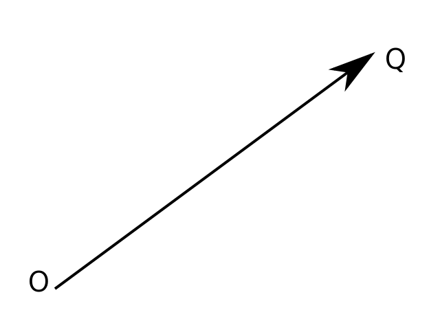
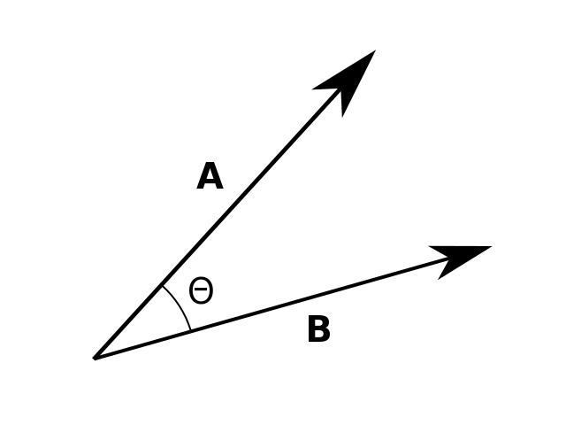
In this tutorial we will examine some of the elementary ideas concerning vectors. The reason for this introduction to vectors is that many concepts in science, for example, displacement, velocity, acceleration, force have a size or magnitude, but also they have associated with them the idea of a direction. And it is obviously more convenient to denote both quantities by just one symbol. That is the vector.

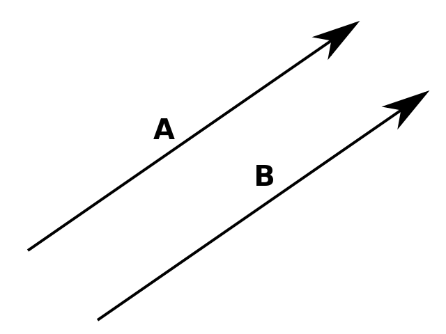
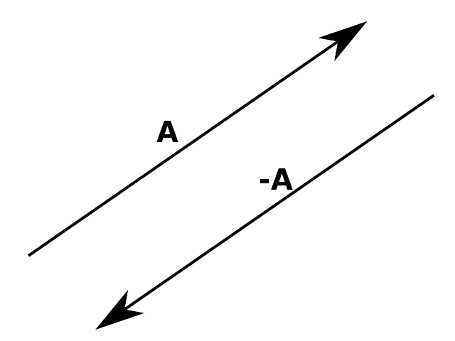
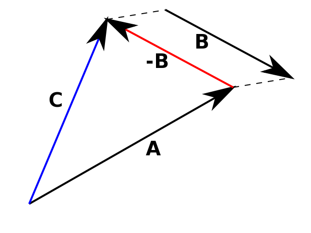
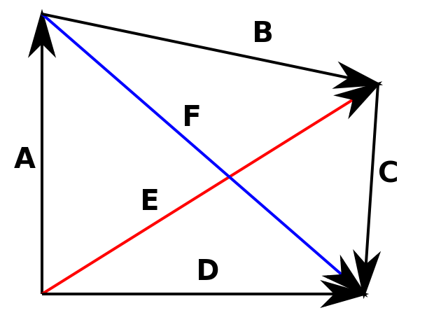
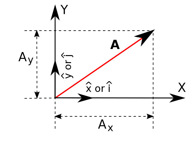
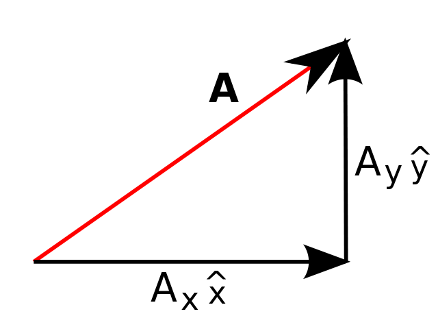
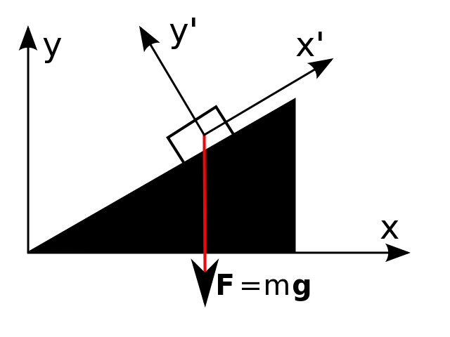
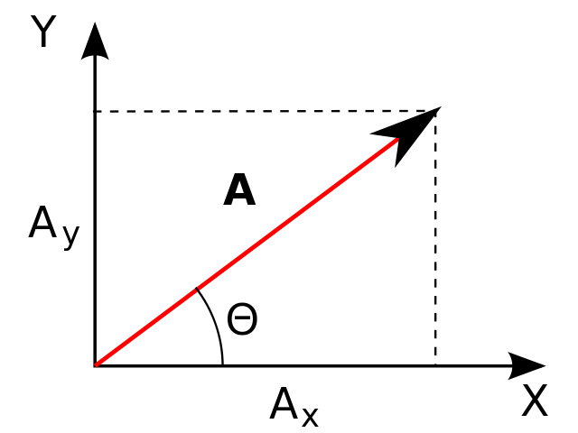
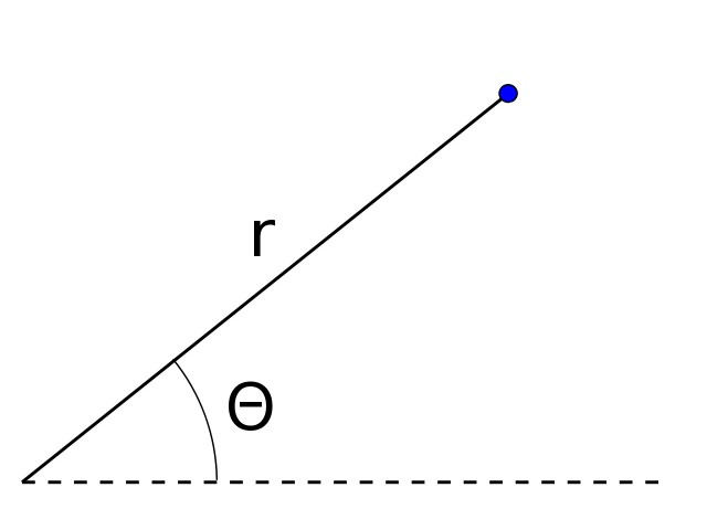
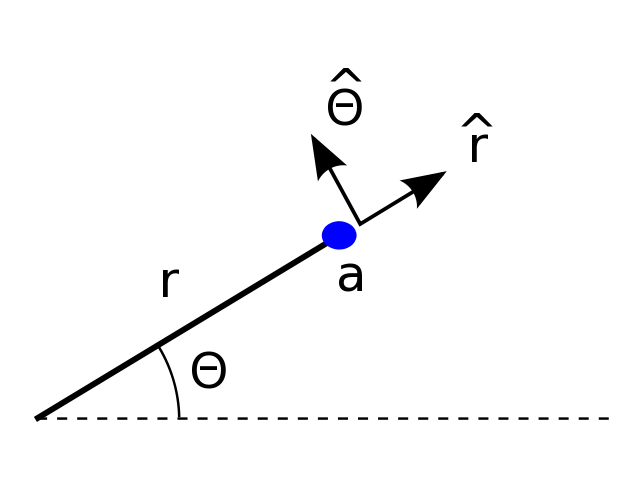
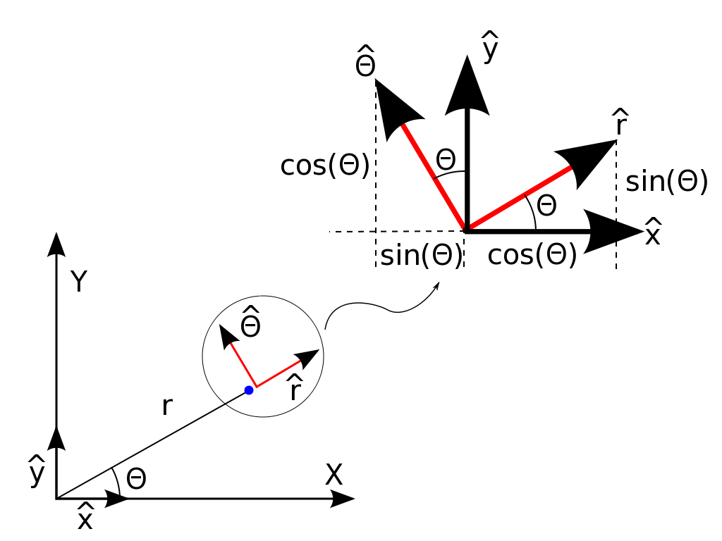
We want you to keep in mind, that vectors are measurable physical quantaties. As such they do not depend on us — observers. In particular, they do not depend on our choice of the coordinate system. However, the way we represent a vector in any given system of coordinates does depend on the coordinate system.

Vectors

Figure 1

Graphically, a vector is represented by an arrow, defining the direction, and the length of the arrow defines the vector's magnitude. This is shown in Fig. 1. If we denote one end of the arrow by the origin O and the tip of the arrow by Q. Then the vector may be represented algebraically by OQ.

This is often simplified to just $\vec{Q}$ or $\bar{Q}$ The arrow and the line above the Q are there to indicate that the symbol represents a vector. Another notation is boldface type as: ${\bf Q}$

Since a direction is implied, ${\bf OQ}\not={\bf QO}$ Even though their lengths are identical, their directions are exactly opposite,in fact ${\bf OQ}=-{\bf QO}$.
The magnitude of a vector is denoted by absolute value signs around the vector symbol: magnitude of ${\bf Q}$ is written as $|{\bf Q}|$ (or magnitude of ${\bf OQ}$ is written as $|{\bf OQ}|$)

There are two fundamental definitions.

Figure 2

Two vectors, $\vec{A}$ and $\vec{B}$ are equal if they have the same magnitude and direction, regardless of whether they have the same initial points, as shown in Figure 2.

Figure 3

A vector having the same magnitude as $\vec{A}$ but the opposite direction is denoted by $-\vec{A}$, as shown in Figure 3.

The operation of addition, subtraction and multiplication of ordinary algebra can be extended to vectors with some new definitions and a few new rules.

Addition and subtraction

Figure 4

We can now define vector addition. The sum of two vectors, $\vec{A}$ and $\vec{B}$, is a vector $\vec{C}$, which is obtained by placing the initial point of $\vec{B}$ on the final point of $\vec{A}$, and then drawing a line from the initial point of $\vec{A}$ to the final point of $\vec{B}$, as illustrated in Figure 4. This is sometimes referred to as the "Tip-to-Tail" method.

The operation of vector addition as described here is written as $\vec{C}=\vec{A}+\vec{B}$.

Vector subtraction is defined in the following way. The difference of two vectors, $\vec{A}-\vec{B}$ , is a vector $\vec{C}$ that is, $\vec{C}=\vec{A}-\vec{B}$ or $\vec{C}=\vec{A}+(-\vec{B})$. Thus vector subtraction can be represented as a vector addition.

Figure 5

The graphical representation is shown in Figure 5. Inspection of the graphical representation shows that we place the initial point of the vector $-\vec{B}$ on the final point the vector $\vec{A}$, and then draw a line from the initial point of $\vec{A}$ to the final point of $-\vec{B}$ to give the difference $\vec{C}$.

This would be a good place to try this simulation on the graphical addition of vectors. Use the "BACK" buttion to return to this point.

Scalars

Any quantity which has a magnitude but no direction associated with it is called a "scalar". For example, speed, mass and temperature. The product of a scalar, $m$ say, times a vector $\vec{A}$, is another vector, $\vec{B}$, where $\vec{B}$ has the same direction as $\vec{A}$ but the magnitude is changed, that is, $|\vec{B}=m|\vec{A}|$.

Vector Algebra

Many of the laws of ordinary algebra hold also for vector algebra. These laws are:

Commutative Law for Addition: $\vec{A}+\vec{B}=\vec{B}+\vec{A}$.
Associative Law for Addition: $\vec{A}+(\vec{B}+\vec{C})=(\vec{A}+\vec{B})+\vec{C}$.
Commutative Law for Multiplication: $m\vec{A}=\vec{A}m$, where $m$ is a scalar.
Associative Law for Multiplication: $(m+n)\vec{A}=m\vec{A}+n\vec{A}$, where $m$ and $n$ are two different scalars.
Distributive Law: $m(\vec{A}+\vec{B})=m\vec{A}+m\vec{B}$.

Proof of the associative law

Associative law is shown in Figure 6.
If we add $\vec{A}$ and $\vec{B}$ and we get a vector $\vec{E}$. And similarly if $\vec{B}$ is added to $\vec{C}$, we get $\vec{F}$. Now $\vec{D}=\vec{E}+\vec{C}=\vec{A}+\vec{F}$. Replacing $\vec{E}$ with $(\vec{A}+\vec{B})$ and $\vec{F}$ with $(\vec{B}+\vec{C})$, we get $\vec{A}+(\vec{B}+\vec{C})=(\vec{A}+\vec{B})+\vec{C}$
The law is verified.

Figure 6

Stop now and make sure that you follow the above proof.
Prove the rest of the laws by yourself.

These laws allow the manipulation of vector quantities in much the same way as ordinary algebraic equations.

Coordinates

Vectors can be related to the basic coordinate systems which we use by the introduction of what we call "unit vectors." A unit vector is one which has a magnitude of $1$ and is often indicated by putting a hat (or circumflex) on top of the vector symbol, for example $\hat{a}$, $|\hat{a}|=1$. I emphasize that $\hat{a}$ is a vector, it has direction. The quantity $\hat{a}$ is read as "a hat" or "a unit".

Figure 7

Let us chose a two-dimensional (or $x$,$y$) Cartesian Coordinate System, as shown in Figure 7.

Important point: Vector represents a physical quantity which exists independent of us. As such vector itself does not depend on our choice of the coordinate system. The coordinates of the vector, however, do depend on the system of coordinates.

Figure 8

We can define a unit vector in the $x$ direction $\hat{x}$, it is also denoted by $\hat{i}$. Similarly in the $y$-direction we use $\hat{y}$ or $\hat{j}$. Any two-dimensional vector can now be represented by employing multiples of the unit vectors, $\hat{x}$ and $\hat{y}$, as illustrated in Figure 8.

The vector A can be represented algebraically by $\vec{A}=\vec{A}_x + \vec{A}_y$. Where $\vec{A}_x$ and $\vec{A}_y$ are vectors in the $x$ and $y$ directions. If $A_x$ and $A_y$ are the magnitudes of $\vec{A}_x$ and $\vec{A}_y$, then $\vec{A}_x=A_x \hat{x}$ and $\vec{A}_y=A_y \hat{j}$. $A_x$ and $A_y$ are called components of vector $\vec{A}$ in $x$ and $y$ directions respectively. Vectors $\vec{A}_x$ and $\vec{A}_y$ are sometimes called vector components of the vector $\vec{A}$.

The vector $\vec{A}$ in the chosen system of coordinates then can be represented as $\vec{A}=A_x \hat{x}+A_y \hat{j}$.

Figure 9

The actual operation implied by this is shown in Figure 9.

Remember: $\hat{x}$ (or $\hat{i}$) and $\hat{y}$ (or $\hat{j}$) have a magnitude of $1$, so they only give a vector its direction.

Resolving a vector

The breaking up of a vector into it's component parts is known as resolving a vector. Notice that the representation of $\vec{A}$ by it's components, $A_x \hat{i}$ and $A_y \hat{j}$ is not unique. Depending on the orientation of the coordinate system with respect to the vector in question, it is possible to have more than one set of components.

It is perhaps easier to understand this by having a look at an example.

Figure 10

Consider an object of mass, $M$, placed on a smooth inclined plane, as shown in Figure 10. The gravitational force acting on the object is a vector $\vec{F}=m\vec{g}$, where $\vec{g}$ is the acceleration of free fall.

In the unprimed coordinate system, the vector $\vec{F}$ can be written as $\vec{F}=-F_y \hat{j}$, but in the primed coordinate system the same vector $\vec{F}=-F_{x'} \vec{i'}+F_{y'}\hat{j'}$.

Again the vector $\vec{F}$ is the same vector in both cases (after all it is a real force!), but our representation of it changed, as we changed the coordinate system. Which representation to use will depend on the particular problem that you are faced with.

For example, if you wish to determine the acceleration of the block down the plane, then you will need the component of the force which acts down the plane. That is, $-F_{x'}\hat{i'}$, which would be equal to the mass times the acceleration.

Components, magnitude and angle

Figure 11

The breaking up of a vector into it's components, makes the determination of the length of the vector quite simple and straight forward.

Since $\vec{A}=A_x \hat{i}+A_y \hat{j}$, then using Pythagorus' Theorem we find the magnitude of the vector $\vec{A}$: $|\vec{A}|=\sqrt{A_x^2+A_y^2}$.

For example, if $\vec{A}=3\hat{i}+4\hat{j}$, then $|\vec{A}|=\sqrt{3^2+4^2}=\sqrt{25}=5 $.

We can also find the angle between the vector $\vec{A}$ and say $x$ direction. From trigonometry we have $\cos (\Theta)=A_x/|\vec{A}|$.

Very often in vector problems you will know the length, that is, the magnitude of the vector and you will also know the direction of the vector. From these you will need to calculate the Cartesian components, that is, the $x$ and $y$ components.

The situation is illustrated in Figure 11. Let us assume that the magnitude of $\vec{A}$ and the angle $\Theta$ are given; what we wish to know is, what are $A_x$ and $A_y$?

Again the same trigonometry gives: $\cos (\Theta)=A_x/|\vec{A}|$ therefore $A_x=|\vec{A}|\cos (\Theta)$, and similarly $A_y=|\vec{A}|\cos (90^\circ-\Theta)=|\vec{A}|\sin (\Theta)$,

Algebraic addition and subtraction

Figure 12

The resolution of a vector into it's components can be used in the addition and subtraction of vectors. To illustrate this let us consider an example, what is the sum of the following three vectors?

\begin{eqnarray} &&\vec{A}=A_x \hat{i}+A_y\hat{j}\\ &&\vec{B}=B_x \hat{i}+B_y\hat{j}\\ &&\vec{C}=C_x \hat{i}+C_y\hat{j} \end{eqnarray}

By resolving each of these three vectors into their components we see that the result is Figure 12.

\begin{eqnarray} &&D_x=A_x+B_x+C_x\\ &&D_y=A_y+B_y+C_y \end{eqnarray}

so for the vector $\vec{D}$ we get $\vec{D}=D_x \hat{i}+D_y\hat{j}$.

Now we can calculate the magnitude of the vector $\vec{D}$, as well as the angle between the vector $\vec{D}$ and, say, $x$ direction.

Can you do that? If you cannot read the previous section!

Now you should use this simulation to study the very important topic of the algebraic addition of vectors (look at the vector's components) Use the "BACK" buttion to return to this point.

Polar Coordinate System

Until now, we have discussed vectors in terms of a Cartesian, that is, an $x$-$y$ coordinate system. Any of the vectors used in this frame of reference were directed along, or referred to, the coordinate axes. However there is another coordinate system which is very often encountered and that is the Polar Coordinate System.

Figure 13

In Polar coordinates one specifies the length of the line and it's orientation with respect to some fixed line. In Figure 13, the position of the dot is specified by it's distance from the origin, that is $r$ , and the position of the line is at some angle $\Theta$, from a fixed line as indicated. The quantities $r$ and $\Theta$ are known as the Polar Coordinate System of the point.

Figure 14

It is possible to define fundamental unit vectors in the Polar Coordinate system in much the same way as for Cartesian coordinates. We require that the unit vectors be perpendicular to one another, and that one unit vector be in the direction of increasing $r$, and that the other is in the direction of increasing $\Theta$.

In Figure 14, we have drawn these two unit vectors with the symbols $\hat{r}$ and $\hat{\Theta}$. It is clear that there must be a relation between these unit vectors and those of the Cartesian system.

Figure 15

These relationships are derived in Figure 15.

\begin{eqnarray} &&\hat{r}=\hat{x}\cos \Theta+\hat{y}\sin \Theta\\ &&\hat{\Theta}=-\hat{x}\sin\Theta+\hat{y}\cos\Theta \end{eqnarray}

And inverse relations:

\begin{eqnarray} &&\hat{x}=\hat{r}\cos \Theta-\hat{\Theta}\sin \Theta\\ &&\hat{y}=\hat{r}\sin\Theta+\hat{\Theta}\cos\Theta \end{eqnarray}

Can you see how these relations were derived? Please, make sure that you do!

Important point: $r$ and $\Theta$ are just numbers — coordinates, while $\hat{r}$ and $\hat{\Theta}$ are unit vectors. Their magnitude is $1$ but they have directions! Do not confuse vectors and numbers.

Scalar product

The multiplication of two vectors, is not uniquely defined, in the sense that there is a question as to whether the product will be a vector or not. For this reason there are two types of vector multiplication.

First, the scalar or dot product of two vectors, which results in a scalar.
And secondly, the vector or cross product of two vectors, which results in a vector.

In this tutorial we discuss only the scalar or dot product.

Figure 16

The scalar product of two vectors, $\vec{A}$ and $\vec{B}$ denoted by $\vec{A}\cdot\vec{B}$, is defined as the product of the magnitudes of the vectors times the cosine of the angle between them $\vec{A}\cdot\vec{B}=|\vec{A}||\vec{B}|\cos \Theta$, as illustrated in Figure 16.

Important note: The result of dot product is a scalar, not a vector. In particular it means that the result of dot product will be independent of what system of coordinate you chose to represent your vectors.

From the definition we find

For any vector $\vec{A}$ its magnitude $|\vec{A}|=\sqrt{\vec{A}\cdot\vec{A}}$, since the angle between a vector and itself is $0$, and the cosine of $0$ is $1$.
For any two nonzero vectors $\vec{A}$ and $\vec{B}$ the angle between them is given by $\cos\Theta=\frac{\vec{A}\cdot\vec{B}}{|\vec{A}||\vec{B}|}$.

The rules for scalar products are given in the following list:

$\vec{A}\cdot\vec{B}=\vec{B}\cdot\vec{A}$
$\vec{A}\cdot \left(\vec{B}+\vec{C}\right)=\vec{A}\cdot \vec{B}+\vec{A}\cdot\vec{C}$
$m\left(\vec{A}\cdot\vec{B}\right)=\left(m\vec{A}\right)\cdot\vec{B}=\vec{A}\cdot\left(m\vec{B}\right)=\left(\vec{A}\cdot\vec{B}\right)m$,

where $m$ is an arbitrary scalar and $\vec{A}$, $\vec{B}$, and $\vec{C}$ are arbitrary vectors.

In particular>

$\hat{x}\cdot\hat{x}=\hat{y}\cdot\hat{y}=1$, since $|\hat{x}|=|\hat{y}|=1$.
$\hat{x}\cdot\hat{y}=0$, since the angle between $\hat{x}$ and $\hat{y}$ is $90^\circ$ and $\cos 90^\circ = 0$.

In general then, if $\vec{A}\cdot\vec{B}=0$ and neither the magnitude of $\vec{A}$ nor $\vec{B}$ is $0$, then $\vec{A}$ and $\vec{B}$ must be perpendicular/orthogonal.

The definition of the scalar product given earlier, requires a knowledge of the magnitude of $\vec{A}$ and $\vec{B}$, as well as the angle between the two vectors. If we are given the vectors in terms of a Cartesian representation, that is, in terms of $x$ and $y$, we can use the information to work out the scalar product, without having to determine the angle between the vectors.

If, \begin{eqnarray} &&\vec{A}=A_x\hat{i}+A_y\hat{j}\\ &&\vec{B}=B_x\hat{i}+B_y\hat{j} \end{eqnarray} then $\vec{A}\cdot\vec{B}=(A_x\hat{i}+A_y\hat{j})\cdot(B_x\hat{i}+B_y\hat{j})= A_xB_x \hat{i}\cdot\hat{i}+A_xB_y \hat{i}\cdot\hat{j}+A_yB_x \hat{j}\cdot\hat{i}+A_yB_y \hat{j}\cdot\hat{j}=A_xB_x+A_yB_y$.

Important note: The coordinates $A_x$, $A_y$, $B_x$, and $B_y$ depend on what system of coordinates you choose, but the combination $A_xB_x+A_yB_y$ will be the independent of the system of coordinates.

Example.

Consider two vectors:

\begin{eqnarray} &&\vec{A}=2\hat{i}+2\hat{j}\\ &&\vec{B}=6\hat{i}-3\hat{j} \end{eqnarray}

What is the angle between these two vectors?

Solution

First, we calculate the magnitudes of the two vectors: $|\vec{A}|=\sqrt{\vec{A}\cdot\vec{A}}=\sqrt{2^2+2^2}=\sqrt{8}\approx 2.83$ and $|\vec{B}|=\sqrt{\vec{B}\cdot\vec{B}}=\sqrt{6^2+(-3)^2}=\sqrt{45}\approx 6.71$.
Second, we calculate the scalar product: $\vec{A}\cdot\vec{B}=2\times 6+2\times (-3)=6$.
Finally, we calculate the cosine of the angle between the two vectors $\cos \Theta = \frac{\vec{A}\cdot\vec{B}}{|\vec{A}||\vec{B}|}=\frac{6}{2.83\times 6.71}\approx 0.316$ and the angle itself $\Theta\approx 71^\circ$..

End note.

This concludes our survey of the elementary properties of vectors, we have concentrated on fundamentals and have restricted ourselves to the discussion of vectors in just two dimensions. Nevertheless, a sound grasp of the ideas presented in this tutorial are absolutely essential for further progress in vector analysis. It is even more important for physics.